Bootstrap aggregating

Bootstrap aggregating, also called bagging (from bootstrap aggregating), is a machine learning ensemble meta-algorithm designed to improve the stability and accuracy of machine learning algorithms used in statistical classification and regression. It also reduces variance and helps to avoid overfitting. Although it is usually applied to decision tree methods, it can be used with any type of method. Bagging is a special case of the model averaging approach.

Description of the technique

Given a standard training set $D$ of size n, bagging generates m new training sets $D_{i}$ , each of size n′, by sampling from D uniformly and with replacement. By sampling with replacement, some observations may be repeated in each $D_{i}$ . If n′=n, then for large n the set $D_{i}$ is expected to have the fraction (1 - 1/e) (≈63.2%) of the unique examples of D, the rest being duplicates.[1] This kind of sample is known as a bootstrap sample. Sampling with replacement ensures each bootstrap is independent from its peers, as it does not depend on previous chosen samples when sampling. Then, m models are fitted using the above m bootstrap samples and combined by averaging the output (for regression) or voting (for classification).

An illustration for the concept of bootstrap aggregating

Bagging leads to "improvements for unstable procedures",[2] which include, for example, artificial neural networks, classification and regression trees, and subset selection in linear regression.[3] Bagging was shown to improve preimage learning.[4][5] On the other hand, it can mildly degrade the performance of stable methods such as K-nearest neighbors.[2]

Process of the algorithm

Key Terms

There are three types of datasets in bootstrap aggregating. These are the original, bootstrap, and out-of-bag datasets. Each section below will explain how each dataset is made except for the original dataset. The original dataset is whatever information is given.

Creating the bootstrap dataset

The bootstrap dataset is made by randomly picking objects from the original dataset. Also, it must be the same size as the original dataset. However, the difference is that the bootstrap dataset can have duplicate objects. Here is simple example to demonstrate how it works along with the illustration below:

Suppose the original dataset is a group of 12 people. These guys are Emily, Jessie, George, Constantine, Lexi, Theodore, John, James, Rachel, Anthony, Ellie, and Jamal.

By randomly picking a group of names, let us say our bootstrap dataset had James, Ellie, Constantine, Lexi, John, Constantine, Theodore, Constantine, Anthony, Lexi, Constantine, and Theodore. In this case, the bootstrap sample contained four duplicates for Constantine, and two duplicates for Lexi, and Theodore.

Creating the out-of-bag dataset

The out-of-bag dataset represents the remaining people who were not in the bootstrap dataset. It can be calculated by taking the difference between the original and the bootstrap datasets. In this case, the remaining samples who were not selected are Emily, Jessie, George, Rachel, and Jamal. Keep in mind that since both datasets are sets, when taking the difference the duplicate names are ignored in the bootstrap dataset. The illustration below shows how the math is done:

Importance

Creating the bootstrap and out-of-bag datasets is crucial since it is used to test the accuracy of a random forest algorithm. For example, a model that produces 50 trees using the bootstrap/out-of-bag datasets will have a better accuracy than if it produced 10 trees. Since the algorithm generates multiple trees and therefore multiple datasets the chance that an object is left out of the bootstrap dataset is low. The next few sections talk about how the random forest algorithm works in more detail.

Creation of Decision Trees

The next step of the algorithm involves the generation of decision trees from the bootstrapped dataset. To achieve this, the process examines each gene/feature and determines for how many samples the feature's presence or absence yields a positive or negative result. This information is then used to compute a confusion matrix, which lists the true positives, false positives, true negatives, and false negatives of the feature when used as a classifier. These features are then ranked according to various classification metrics based on their confusion matrices. Some common metrics include estimate of positive correctness (calculated by subtracting false positives from true positives), measure of "goodness", and information gain. These features are then used to partition the samples into two sets: those who possess the top feature, and those who do not.

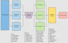
The diagram below shows a decision tree of depth two being used to classify data. For example, a data point that exhibits Feature 1, but not Feature 2, will be given a "No". Another point that does not exhibit Feature 1, but does exhibit Feature 3, will be given a "Yes".

This process is repeated recursively for successive levels of the tree until the desired depth is reached. At the very bottom of the tree, samples that test positive for the final feature are generally classified as positive, while those that lack the feature are classified as negative.[6] These trees are then used as predictors to classify new data.

Random Forests

The next part of the algorithm involves introducing yet another element of variability amongst the bootstrapped trees. In addition to each tree only examining a bootstrapped set of samples, only a small but consistent number of unique features are considered when ranking them as classifiers. This means that each tree only knows about the data pertaining to a small constant number of features, and a variable number of samples that is less than or equal to that of the original dataset. Consequently, the trees are more likely to return a wider array of answers, derived from more diverse knowledge. This results in a random forest, which possesses numerous benefits over a single decision tree generated without randomness. In a random forest, each tree "votes" on whether or not to classify a sample as positive based on its features. The sample is then classified based on majority vote. An example of this is given in the diagram below, where the four trees in a random forest vote on whether or not a patient with mutations A, B, F, and G has cancer. Since three out of four trees vote yes, the patient is then classified as cancer positive.

Because of their properties, random forests are considered one of the most accurate data mining algorithms, are less likely to overfit their data, and run quickly and efficiently even for large datasets.[7] They are primarily useful for classification as opposed to regression, which attempts to draw observed connections between statistical variables in a dataset. This makes random forests particularly useful in such fields as banking, healthcare, the stock market, and e-commerce where it is important to be able to predict future results based on past data.[8] One of their applications would be as a useful tool for predicting cancer based on genetic factors, as seen in the above example.

There are several important factors to consider when designing a random forest. If the trees in the random forests are too deep, overfitting can still occur due to over-specificity. If the forest is too large, the algorithm may become less efficient due to an increased runtime. Random forests also do not generally perform well when given sparse data with little variability.[8] However, they still have numerous advantages over similar data classification algorithms such as neural networks, as they are much easier to interpret and generally require less data for training.[9] As an integral component of random forests, bootstrap aggregating is very important to classification algorithms, and provides a critical element of variability that allows for increased accuracy when analyzing new data, as discussed below.

Wisdom of Crowds

One key component to generating an accurate decision tree and random forest is utilizing the wisdom of crowds. The wisdom of crowds is the collective opinion of a group of individuals rather than that of a single expert.[10] Utilizing the wisdom of crowds allows for the random forest developed from multiple decision trees to be accurate. When building a random forest, each decision tree acts as a person in the crowd. One decision tree's outcome is not dependent upon the outcome of the next when generating a random forest, they are created independently with a randomized subset of data from a shared set of mutations and or samples. Each of the generated trees determines a vote and averaging these results will determine the result per the wisdom of the crowd.

In order to implement this method effectively, the crowd (decision trees) must include the prerequisite qualities as listed below in the table.

5 Qualities Necessary For A Wise Crowd[11]
Criteria	General Description	Random Forest Connection
Diversity of Opinion	Each person should have private information even if it is just an eccentric interpretation of the known facts.	The mutations and samples are the known data that each tree in the forest shares. The votes developed by each tree are "private" information until aggregation of all decision tree results happen. The randomized subsets of the shared data are also "private."
Independence	People's opinions are not determined by the opinions of those around them.	Each decision tree that is built is independent with its own randomly selected subset of data. This randomized subset of each tree is not influenced by the subsets from the other trees.
Decentralization	People are able to specialize and draw on their local knowledge.	Instead of the decision trees forming their results based on the results of other decision trees, they draw upon the results from their specific data set to determine the accurate result.
Aggregation	Some mechanism exists for turning private judgements into a collective decision.	Each tree returns its own results which allow for the collective results from each tree to be compared for a final result.
Trust	Each person trusts the collective group to be fair and valid.	Trust in a random forest refers to the belief that each decision tree generated, and each individual result are accurate alone, and as a collective group the aggregation of all of their results is also accurate.

**This table defines the 5 necessary criteria for generating a random forest with a wise crowd.**

The wisdom of crowds when the above criteria are met yields a wise judgement. However, there are situations where the wisdom of the crowd is not accurate and produces a failed judgement. Some examples of crowds that create a failed judgement: mobs, citizens experiencing a market crash, etc. Wisdom of crowds is not only useful for generating decision trees but can also be used by businesses for marketing purposes, for generating social data analysis, and more. Generating and studying the wisdom of crowds in a random forest is an accurate way to judge the overall determining result. Below is a simple example of how the wisdom of crowd functions in a given random forest generation.

In this example, the result that needs to be determined is whether or not it is summer. This a dataset of temperatures over the course of a month: [76, 82, 69, 67, 87, 70, 66, 42, 48, 51, 62, 65, 74, 88, 90, 59, 67, 49, 52, 67, 63, 64, 67, 77, 75, 65, 55, 91]. This is the dataset used to make the subset of 12 temperatures for each decision tree. In this example, there are 3 generated trees (3 randomized subsets of temperatures). The graphic below displays Decision Tree 1, its subset, along with explanations of how the tree makes its decision and comes to a result.

Decision Tree 1 Diagram with Labeled Decisions

Wisdom of Crowds Example Including Decisions

Temperature 77 in Tree 1 answers yes to the Decision 1, moving to the left to Decision 2. Then at Decision 2, it also answers yes which takes it to the left-most branch of the tree. This is the same process used to build the other two decision trees (people) with each temperature from the subset. The 3 generated trees serve as the crowd in this example. Tree 1 as shown above returned the vote "Yes" for whether or not it is summer based on the results with the majority of data from the subset evaluating the decision as yes. The results from this crowd are shown in the image below. Green represents the “Yes” temperatures of each subset and the pink represents the "No" temperatures based on each decision criterion.

Final Decision Tree Results:

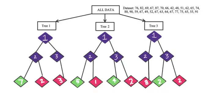
Completed Random Forest - Wisdom of Crowds Example

Looking at the generated votes from each tree(person) in the example above, in trees 1 and 2, it was voted to be summer. In tree 3, the decision was determined to be no. The aggregation of the results from each tree returns "Yes" for summer 2 out of 3 times, the majority of the time. The crowd in this example indicates that the overall result is yes. This means that the random forest generated a final result that it is in fact summer.

This simple example displays how the aggregation of each decision tree’s results leads to one final decision based on the wisdom of the crowd. The way each decision tree is built follows the criteria set in the table.

Utilizing the wisdom of crowds creates a diverse set of data. This is what allows random forests to be highly accurate. Without following the criteria explained in this section, generated random forests could not be trusted to generate accurate decisions of data of any kind. This is one of the most important aspects to consider and improve when creating and evaluating any data using decision trees and a random forest. The next section will cover ways to improve random forests with characteristics in addition to the wisdom of crowds.

Improving Random Forests and Bagging

While the techniques described above to utilize random forests, bagging (otherwise known as bootstrapping), and wisdom of crowds are incredibly useful on their own, there are certain methods that can be used in order to improve their execution and voting time, their prediction accuracy, and their overall performance. The following are key steps in creating an efficient random forest:

Specify the maximum depth of trees: Instead of allowing your random forest to continue until all nodes are pure, it is better to cut it off at a certain point in order to further decrease chances of overfitting.
Prune the dataset: Using an extremely large dataset may prove to create results that is less indicative of the data provided than a smaller set that more accurately represents what is being focused on.
- Continue pruning the data at each node split rather than just in the original bagging process.
Decide on accuracy or speed: Depending on the desired results, increasing or decreasing the number of trees within the forest can help. Increasing the number of trees generally provides more accurate results while decreasing the number of trees will provide quicker results.

Pros and Cons of Random Forests and Bagging
Pros	Cons
There are overall less requirements involved for normalization and scaling, making the use of random forests more convenient.[12]	The algorithm may change significantly if there is a slight change to the data being bootstrapped and used within the forests.[13] In other words, random forests are incredibly dependent on their data sets, changing these can drastically change the individual trees' structures.
Easy data preparation. Data is prepared by creating a bootstrap set and a certain number of decision trees to build a random forest that also utilizes feature selection, as mentioned in the Random Forests section.	Random Forests are more complex to implement than lone decision trees or other algorithms. This is because they take extra steps for bagging, as well as the need for recursion in order to produce an entire forest, which complicates implementation. Because of this, it requires much more computational power and computational resources.
Consisting of multiple decision trees, forests are able to more accurately make predictions. Making predictions based on the wisdom of crowds is much more accurate. For example, having one person vote for the president less accurately depicts the truth of opinion than having all people vote.	Requires much more time to train the data compared to decision trees. Having a large forest can quickly begin to decrease the speed in which one's program operates because it has to traverse much more data even though each tree is using a smaller set of samples and features.
Works well with non-linear data. Non-linear data is data that does not involve a single level, meaning it cannot be traversed in one go. Working well with non-linear data is a huge advantage because other data mining techniques such as single decision trees do not handle this as well.	Requires much more time to make decisions and vote within the random forest classifier. The random forest classifier need to vote using wisdom of crowds, which takes much more time than classifying within a single decision tree.
There is a lower risk of overfitting and runs efficiently on even large data sets.[14] This is the result of the random forest's use of bagging in conjunction with random feature selection.	Does not predict beyond the range of the training data. This is a con because while bagging is often effective, all of the data is not being considered, therefore it cannot predict an entire dataset.
The random forest classifier operates with a high accuracy and speed.[15] Random forests are much faster than decision trees because of using a smaller data set.	To recreate specific results you need to keep track of the exact random seed used to generate the bootstrap sets. This may be important when collecting data for research or within a data mining class. Using random seeds is essential to the random forests, but can make it hard to support your statements based on forests if there is a failure to record the seeds.
Deals with missing data and datasets with many outliers well. They deal with this by using binning, or by grouping values together to avoid values that are terribly far apart.

Algorithm (classification)

Flow chart of the bagging algorithm when used for classification

For classification, use a training set $D$ , Inducer $I$ and the number of bootstrap samples $m$ as input. Generate a classifier $C^{*}$ as output[16]

Create $m$ new training sets $D_{i}$ , from $D$ with replacement
Classifier $C_{i}$ is built from each set $D_{i}$ using $I$ to determine the classification of set $D_{i}$
Finally classifier $C^{*}$ is generated by using the previously created set of classifiers $C_{i}$ on the original data set $D$ , the classification predicted most often by the sub-classifiers $C_{i}$ is the final classification

for i = 1 to m {
    D' = bootstrap sample from D    (sample with replacement)
    Ci = I(D')
}
C*(x) = argmax #{i:Ci(x)=y}         (most often predicted label y)
         y∈Y

Example: ozone data

To illustrate the basic principles of bagging, below is an analysis on the relationship between ozone and temperature (data from Rousseeuw and Leroy (1986), analysis done in R).

The relationship between temperature and ozone appears to be nonlinear in this data set, based on the scatter plot. To mathematically describe this relationship, LOESS smoothers (with bandwidth 0.5) are used. Rather than building a single smoother for the complete data set, 100 bootstrap samples were drawn. Each sample is composed of a random subset of the original data and maintains a semblance of the master set’s distribution and variability. For each bootstrap sample, a LOESS smoother was fit. Predictions from these 100 smoothers were then made across the range of the data. The black lines represent these initial predictions. The lines lack agreement in their predictions and tend to overfit their data points: evident by the wobbly flow of the lines.

By taking the average of 100 smoothers, each corresponding to a subset of the original data set, we arrive at one bagged predictor (red line). The red line's flow is stable and does not overly conform to any data point(s).

Advantages and disadvantages

Advantages:

Many weak learners aggregated typically outperform a single learner over the entire set, and has less overfit
Removes variance in high-variance low-bias weak learner [17]
Can be performed in parallel, as each separate bootstrap can be processed on its own before combination[18]

Disadvantages:

For weak learner with high bias, bagging will also carry high bias into its aggregate[17]
Loss of interpretability of a model.
Can be computationally expensive depending on the data set

History

The concept of bootstrap aggregating is derived from the concept of bootstrapping which was developed by Bradley Efron.[19] Bootstrap aggregating was proposed by Leo Breiman who also coined the abbreviated term "bagging" (bootstrap aggregating). Breiman developed the concept of bagging in 1994 to improve classification by combining classifications of randomly generated training sets. He argued, "If perturbing the learning set can cause significant changes in the predictor constructed, then bagging can improve accuracy".[3]

References

Aslam, Javed A.; Popa, Raluca A.; and Rivest, Ronald L. (2007); On Estimating the Size and Confidence of a Statistical Audit, Proceedings of the Electronic Voting Technology Workshop (EVT '07), Boston, MA, August 6, 2007. More generally, when drawing with replacement n′ values out of a set of n (different and equally likely), the expected number of unique draws is $n(1-e^{-n'/n})$ .
Breiman, Leo (1996). "Bagging predictors". Machine Learning. 24 (2): 123–140. CiteSeerX 10.1.1.32.9399. doi:10.1007/BF00058655. S2CID 47328136.
Breiman, Leo (September 1994). "Bagging Predictors" (PDF). Technical Report. Department of Statistics, University of California Berkeley (421). Retrieved 2019-07-28.
Sahu, A., Runger, G., Apley, D., Image denoising with a multi-phase kernel principal component approach and an ensemble version, IEEE Applied Imagery Pattern Recognition Workshop, pp.1-7, 2011.
Shinde, Amit, Anshuman Sahu, Daniel Apley, and George Runger. "Preimages for Variation Patterns from Kernel PCA and Bagging." IIE Transactions, Vol.46, Iss.5, 2014
"Decision tree learning", Wikipedia, 2021-11-29, retrieved 2021-11-29
"Random forests - classification description". www.stat.berkeley.edu. Retrieved 2021-12-09.
"Introduction to Random Forest in Machine Learning". Engineering Education (EngEd) Program | Section. Retrieved 2021-12-09.
Montantes, James (2020-02-04). "3 Reasons to Use Random Forest Over a Neural Network–Comparing Machine Learning versus Deep…". Medium. Retrieved 2021-12-09.
"Wisdom of the crowd", Wikipedia, 2021-12-10, retrieved 2021-12-10
"The Wisdom of Crowds", Wikipedia, 2021-10-10, retrieved 2021-12-10
"Random Forest Pros & Cons". HolyPython.com. Retrieved 2021-11-26.
K, Dhiraj (2020-11-22). "Random Forest Algorithm Advantages and Disadvantages". Medium. Retrieved 2021-11-26.
Team, Towards AI. "Why Choose Random Forest and Not Decision Trees – Towards AI — The World's Leading AI and Technology Publication". Retrieved 2021-11-26.
"Random Forest". Corporate Finance Institute. Retrieved 2021-11-26.
Bauer, Eric; Kohavi, Ron (1999). "An Empirical Comparison of Voting Classification Algorithms: Bagging, Boosting, and Variants". Machine Learning. 36: 108–109. doi:10.1023/A:1007515423169. S2CID 1088806. Retrieved 6 December 2020.
"What is Bagging (Bootstrap Aggregation)?". CFI. Corporate Finance Institute. Retrieved December 5, 2020.
Zoghni, Raouf (September 5, 2020). "Bagging (Bootstrap Aggregating), Overview". The Startup – via Medium.
Efron, B. (1979). "Bootstrap methods: Another look at the jackknife". The Annals of Statistics. 7 (1): 1–26. doi:10.1214/aos/1176344552.