Attention (machine learning)
In neural networks, attention is a technique that mimics cognitive attention. The effect enhances some parts of the input data while diminishing other parts — the thought being that the network should devote more focus to that small but important part of the data. Learning which part of the data is more important than others depends on the context and is trained by gradient descent.
Attention-like mechanisms were introduced in the 1990s under names like multiplicative modules, sigma pi units, and hypernetworks.[1] Its flexibility comes from its role as "soft weights" that can change during runtime, in contrast to standard weights that must remain fixed at runtime. Uses of attention include memory in neural Turing machines, reasoning tasks in differentiable neural computers,[2] language processing in transformers, and multi-sensory data processing (sound, images, video, and text) in perceivers.[3][4][5][6]
A language translation example
To build a machine that translates English-to-French (see diagram below), one starts with an Encoder-Decoder and grafts an attention unit to it. In the simplest case such as the example below, the attention unit is just lots of dot products of recurrent layer states and does not need training. In practice, the attention unit consists of 3 fully connected neural network layers that needs to be trained. The 3 layers are called Query, Key, and Value.
 Encoder-Decoder with attention. This diagram uses specific values to relieve an already cluttered notation alphabet soup. The left part (in black) is the Encoder-Decoder, the middle part (in orange) is the attention unit, and the right part (in grey & colors) is the computed data. Grey regions in H matrix and w vector are zero values. Numerical subscripts are examples of vector sizes. Lettered subscripts i and i-1 indicate time step.
|
||||||||||||||||||||||||||||||||
|
This table shows the calculations at each time step. For clarity, it uses specific numerical values and shapes rather than letters. The nested shapes depict the summarizing nature of h, where each h contains a history of the words that came before it. Here, the attention scores were cooked up to get the desired attention weights.
| step | x | h, H = encoder output these are 500x1 vectors represented as shapes | s = decoder input to Attention | alignment score | w = attention weight = softmax( score ) | c = context vector = H*w | y = decoder output |
| 1 | I | - | - | - | - | - | |
| 2 | love | - | - | - | - | - | |
| 3 | you | - | - | - | - | - | |
| 4 | - | - | the decoder state does not exist yet so we use the encoder output h3 to kick off the decoder | [.63 -3.2 -2.5 .5 .5 ...] | [.94 .02 .04 0 0 ...] | .94 * | je |
| 5 | - | - | s4 | [-1.5 -3.9 .57 .5 .5 ...] | [.11 .01 .88 0 0 ...] | .11 * | t' |
| 6 | - | - | s5 | [-2.8 .64 -3.2 .5 .5 ...] | [.03 .95 .02 0 0 ...] | .03 * | aime |
Viewed as a matrix, the attention weights show how the network adjusts its focus according to context.
| I | love | you | |
| je | .94 | .02 | .04 |
| t' | .11 | .01 | .88 |
| aime | .03 | .95 | .02 |
This view of the attention weights addresses the "explainability" problem that neural networks are criticized for. Networks that perform verbatim translation without regard to word order would have a diagonally dominant matrix if they were analyzable in these terms. The off-diagonal dominance shows that the attention mechanism is more nuanced. On the first pass through the decoder, 94% of the attention weight is on the first English word "I", so the network offers the word "je". On the second pass of the decoder, 88% of the attention weight is on the third English word "you", so it offers "t'". On the last pass, 95% of the attention weight is on the second English word "love", so it offers "aime".
Variants
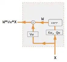
There are many variants of attention: dot product, query-key-value, hard, soft, self, cross, Luong, and Bahdanau to name a few. These variants recombine the encoder-side inputs to redistribute those effects to each target output. Often, a correlation-style matrix of dot products provides the re-weighting coefficients (see legend).
| 1. encoder-decoder dot product | 2. encoder-decoder QKV | 3. encoder-only dot product | 4. encoder-only QKV | 5. Pytorch tutorial |
|---|---|---|---|---|
 Both Encoder & Decoder are needed to calculate Attention.[8] |
 Both Encoder & Decoder are needed to calculate Attention.[9] |
 Decoder is NOT used to calculate Attention. With only 1 input into corr, W is an auto-correlation of dot products. wij = xi * xj [10] |
 Decoder is NOT used to calculate Attention.[11] |
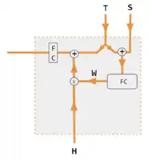 A FC layer is used to calculate Attention instead of dot product correlation.
[12] |
| label | description |
|---|---|
| variables X,H,S,T | upper case variables represent the entire sentence, and not just the current word. For example, H is a matrix of the encoder hidden state—one word per column. |
| S, T | S = decoder hidden state, T = target word embedding. In the Pytorch Tutorial variant training phase, T alternates between 2 sources depending on the level of teacher forcing used. T could be the embedding of the network's output word, i.e. embedding(argmax(FC output)). Alternatively with teacher forcing, T could be the embedding of the known correct word which can occur with a constant forcing probability, say 1/2. |
| X, H | H = encoder hidden state, X = input word embeddings |
| W | attention coefficients |
| Qw, Kw, Vw, FC | weight matrices for query, key, vector respectively. FC is a fully connected weight matrix. |
| circled +, circled x | circled + = vector concatenation. circled x = matrix multiplication |
| corr | column wise softmax( matrix of all combinations of dot products ). The dot products are xi * xj in variant # 3, hi * sj in variant 1, and column i ( Kw*H ) * column j ( Qw*S ) in variant 2, and column i (Kw*X) * column j (Qw*X) in variant 4. variant 5 uses a fully connected layer to determine the coefficients. If the variant is QKV, then the dot products are normalized by the sqrt(d) where d is the height of the QKV matrices. |
See also
- Transformer (machine learning model) § Scaled dot-product attention
- Perceiver § Components for query-key-value (QKV) attention
References
- Yann Lecun (2020). Deep Learning course at NYU, Spring 2020, video lecture Week 6. Event occurs at 53:00. Retrieved 2022-03-08.
- Graves, Alex; Wayne, Greg; Reynolds, Malcolm; Harley, Tim; Danihelka, Ivo; Grabska-Barwińska, Agnieszka; Colmenarejo, Sergio Gómez; Grefenstette, Edward; Ramalho, Tiago; Agapiou, John; Badia, Adrià Puigdomènech; Hermann, Karl Moritz; Zwols, Yori; Ostrovski, Georg; Cain, Adam; King, Helen; Summerfield, Christopher; Blunsom, Phil; Kavukcuoglu, Koray; Hassabis, Demis (2016-10-12). "Hybrid computing using a neural network with dynamic external memory". Nature. 538 (7626): 471–476. Bibcode:2016Natur.538..471G. doi:10.1038/nature20101. ISSN 1476-4687. PMID 27732574. S2CID 205251479.
- Vaswani, Ashish; Shazeer, Noam; Parmar, Niki; Uszkoreit, Jakob; Jones, Llion; Gomez, Aidan N.; Kaiser, Lukasz; Polosukhin, Illia (2017-12-05). "Attention Is All You Need". arXiv:1706.03762 [cs.CL].
- Ramachandran, Prajit; Parmar, Niki; Vaswani, Ashish; Bello, Irwan; Levskaya, Anselm; Shlens, Jonathon (2019-06-13). "Stand-Alone Self-Attention in Vision Models". arXiv:1906.05909 [cs.CV].
- Jaegle, Andrew; Gimeno, Felix; Brock, Andrew; Zisserman, Andrew; Vinyals, Oriol; Carreira, Joao (2021-06-22). "Perceiver: General Perception with Iterative Attention". arXiv:2103.03206 [cs.CV].
- Ray, Tiernan. "Google's Supermodel: DeepMind Perceiver is a step on the road to an AI machine that could process anything and everything". ZDNet. Retrieved 2021-08-19.
- "Pytorch.org seq2seq tutorial". Retrieved December 2, 2021.
- Luong, Minh-Thang (2015-09-20). "Effective Approaches to Attention-based Neural Machine Translation". arXiv:1508.04025v5 [cs.CL].
- Neil Rhodes (2021). CS 152 NN—27: Attention: Keys, Queries, & Values. Event occurs at 06:30. Retrieved 2021-12-22.
- Alfredo Canziani & Yann Lecun (2021). NYU Deep Learning course, Spring 2020. Event occurs at 05:30. Retrieved 2021-12-22.
- Alfredo Canziani & Yann Lecun (2021). NYU Deep Learning course, Spring 2020. Event occurs at 20:15. Retrieved 2021-12-22.
- Robertson, Sean. "NLP From Scratch: Translation With a Sequence To Sequence Network and Attention". pytorch.org. Retrieved 2021-12-22.
External links
- Dan Jurafsky and James H. Martin (2022) Speech and Language Processing (3rd ed. draft, January 2022), ch. 10.4 Attention and ch. 9.7 Self-Attention Networks: Transformers
- Alex Graves (4 May 2020), Attention and Memory in Deep Learning (video lecture), DeepMind / UCL, via YouTube
- Rasa Algorithm Whiteboard - Attention via YouTube
Differentiable computing | |||||||
|---|---|---|---|---|---|---|---|
| General | |||||||
| Concepts | |||||||
| Programming languages | |||||||
| Application | |||||||
| Hardware | |||||||
| Software library | |||||||
| Implementation |
| ||||||
| People | |||||||
| Organizations | |||||||
| |||||||