Dixon elliptic functions

In mathematics, the Dixon elliptic functions sm and cm are two elliptic functions (doubly periodic meromorphic functions on the complex plane) that map from each regular hexagon in a hexagonal tiling to the whole complex plane. Because these functions satisfy the identity $\operatorname {cm} ^{3}z+\operatorname {sm} ^{3}z=1$ , as real functions they parametrize the cubic Fermat curve $x^{3}+y^{3}=1$ , just as the trigonometric functions sine and cosine parametrize the unit circle $x^{2}+y^{2}=1$ .

The Dixon elliptic functions cm, sm applied to a real-valued argument x. Both functions are periodic with real period

\pi _{3}\approx 5.29991625

\operatorname {sm} z

in the complex plane, illustrating its double periodicity (

\omega =e^{2\pi i/3}

).[1]

They were named sm and cm by Alfred Dixon in 1890, by analogy to the trigonometric functions sine and cosine and the Jacobi elliptic functions sn and cn; Göran Dillner described them earlier in 1873.[2]

Definition

The functions sm and cm can be defined as the solutions to the initial value problem:[3]

{\frac {d}{dz}}\operatorname {cm} z=-\operatorname {sm} ^{2}z,\ {\frac {d}{dz}}\operatorname {sm} z=\operatorname {cm} ^{2}z,\ \operatorname {cm} (0)=1,\ \operatorname {sm} (0)=0

Or as the inverse of the Schwarz–Christoffel mapping from the complex unit disk to an equilateral triangle, the Abelian integral:[4]

z=\int _{0}^{\operatorname {sm} z}{\frac {dw}{(1-w^{3})^{2/3}}}=\int _{\operatorname {cm} z}^{1}{\frac {dw}{(1-w^{3})^{2/3}}}

which can also be expressed using the hypergeometric function:[5]

\operatorname {sm} ^{-1}(z)=z\,{}_{2}F_{1}\left({\frac {1}{3}},{\frac {2}{3}};{\frac {4}{3}};z^{3}\right)

Parametrization of the cubic Fermat curve

The function

t\mapsto (\operatorname {cm} t,\operatorname {sm} t)

parametrizes the cubic Fermat curve, with area of the sector equal to half the argument

t

.

Both sm and cm have a period along the real axis of $\pi _{3}=\mathrm {B} {\bigl (}{\tfrac {1}{3}},{\tfrac {1}{3}}{\bigr )}={\tfrac {\sqrt {3}}{2\pi }}\Gamma ^{3}{\bigl (}{\tfrac {1}{3}}{\bigr )}\approx 5.29991625$ with $\mathrm {B}$ the beta function and $\Gamma$ the gamma function:[6]

{\begin{aligned}{\tfrac {1}{3}}\pi _{3}&=\int _{-\infty }^{0}{\frac {dx}{(1-x^{3})^{2/3}}}=\int _{0}^{1}{\frac {dx}{(1-x^{3})^{2/3}}}=\int _{1}^{\infty }{\frac {dx}{(1-x^{3})^{2/3}}}\\[8mu]&\approx 1.76663875\end{aligned}}

They satisfy the identity $\operatorname {cm} ^{3}z+\operatorname {sm} ^{3}z=1$ . The parametric function $t\mapsto (\operatorname {cm} t,\,\operatorname {sm} t),$ $t\in {\bigl [}{-{\tfrac {1}{3}}}\pi _{3},{\tfrac {2}{3}}\pi _{3}{\bigr ]}$ parametrizes the cubic Fermat curve $x^{3}+y^{3}=1,$ with ${\tfrac {1}{2}}t$ representing the signed area lying between the segment from the origin to $(1,\,0)$ , the segment from the origin to $(\operatorname {cm} t,\,\operatorname {sm} t)$ , and the Fermat curve, analogous to the relationship between the argument of the trigonometric functions and the area of a sector of the unit circle.[7] To see why, apply Green's theorem:

A={\tfrac {1}{2}}\int _{0}^{t}(x\mathop {dy} -y\mathop {dx} )={\tfrac {1}{2}}\int _{0}^{t}(\operatorname {cm} ^{3}t+\operatorname {sm} ^{3}t)\mathop {dt} ={\tfrac {1}{2}}\int _{0}^{t}dt={\tfrac {1}{2}}t.

Notice that the area between the $x+y=0$ and $x^{3}+y^{3}=1$ can be broken into three pieces, each of area ${\tfrac {1}{6}}\pi _{3}$ :

{\begin{aligned}{\tfrac {1}{2}}\pi _{3}&=\int _{-\infty }^{\infty }{\bigl (}(1-x^{3})^{1/3}+x{\bigr )}\mathop {dx} \\[8mu]{\tfrac {1}{6}}\pi _{3}&=\int _{-\infty }^{0}{\bigl (}(1-x^{3})^{1/3}+x{\bigr )}\mathop {dx} =\int _{0}^{1}(1-x^{3})^{1/3}\mathop {dx} .\end{aligned}}

Symmetries

The function $\operatorname {sm} z$ has zeros at the complex-valued points $z={\tfrac {1}{\sqrt {3}}}\pi _{3}i(a+b\omega )$ for any integers $a$ and $b$ , where $\omega$ is a cube root of unity, $\omega =\exp {\tfrac {2}{3}}i\pi =-{\tfrac {1}{2}}+{\tfrac {\sqrt {3}}{2}}i$ (that is, $a+b\omega$ is an Eisenstein integer). The function $\operatorname {cm} z$ has zeros at the complex-valued points $z={\tfrac {1}{3}}\pi _{3}+{\tfrac {1}{\sqrt {3}}}\pi _{3}i(a+b\omega )$ . Both functions have poles at the complex-valued points $z=-{\tfrac {1}{3}}\pi _{3}+{\tfrac {1}{\sqrt {3}}}\pi _{3}i(a+b\omega )$ .

Fundamental reflections, rotations, and translations

\operatorname {cm} {\bar {z}}={\overline {\operatorname {cm} z}}

\operatorname {sm} {\bar {z}}={\overline {\operatorname {sm} z}}

\operatorname {cm} (-z)={\frac {1}{\operatorname {cm} z}}=\operatorname {sm} {\bigl (}z+{\tfrac {1}{3}}\pi _{3}{\bigr )}

\operatorname {sm} (-z)=-{\frac {\operatorname {sm} z}{\operatorname {cm} z}}={\frac {1}{\operatorname {sm} {\bigl (}z-{\tfrac {1}{3}}\pi _{3}{\bigr )}}}=\operatorname {cm} {\bigl (}z+{\tfrac {1}{3}}\pi _{3}{\bigr )}

\operatorname {cm} \omega z=\operatorname {cm} z=\operatorname {cm} \omega ^{2}z

\operatorname {sm} \omega z=\omega \operatorname {sm} z=\omega ^{2}\operatorname {sm} \omega ^{2}z

\operatorname {cm} {\bigl (}z+\pi _{3}(a+b\omega ){\bigr )}=\operatorname {cm} z

\operatorname {sm} {\bigl (}z+\pi _{3}(a+b\omega ){\bigr )}=\operatorname {sm} z,

where

a+b\omega

is any Eisenstein integer.

Specific values

\operatorname {cm} {\bigl (}{-{\tfrac {1}{3}}}\pi _{3}{\bigr )}=\operatorname {sm} {\bigl (}{-{\tfrac {1}{3}}}\pi _{3}{\bigr )}=\infty

\operatorname {cm} (0)=\operatorname {sm} {\bigl (}{\tfrac {1}{3}}\pi _{3}{\bigr )}=1

\operatorname {cm} {\bigl (}{\tfrac {1}{3}}\pi _{3}{\bigr )}=\operatorname {sm} (0)=0

\operatorname {cm} {\bigl (}{\tfrac {1}{2}}\pi _{3}{\bigr )}=\operatorname {sm} {\bigl (}{-{\tfrac {1}{6}}}\pi _{3}{\bigr )}=-1

\operatorname {cm} {\bigl (}{\tfrac {1}{6}}\pi _{3}{\bigr )}=\operatorname {sm} {\bigl (}{\tfrac {1}{6}}\pi _{3}{\bigr )}=2^{-1/3}

\operatorname {cm} {\bigl (}{-{\tfrac {1}{6}}}\pi _{3}{\bigr )}=\operatorname {sm} {\bigl (}{\tfrac {1}{2}}\pi _{3}{\bigr )}=2^{1/3}

Sum and difference identities

The Dixon elliptic functions satisfy the argument sum and difference identities:[8]

{\begin{aligned}\operatorname {cm} (u+v)&={\frac {\operatorname {sm} u\,\operatorname {cm} u-\operatorname {sm} v\,\operatorname {cm} v}{\operatorname {sm} u\,\operatorname {cm} ^{2}v-\operatorname {cm} ^{2}u\,\operatorname {sm} v}}\\[8mu]\operatorname {cm} (u-v)&={\frac {\operatorname {cm} ^{2}u\,\operatorname {cm} v-\operatorname {sm} u\,\operatorname {sm} ^{2}v}{\operatorname {cm} u\,\operatorname {cm} ^{2}v-\operatorname {sm} ^{2}u\,\operatorname {sm} v}}\\[8mu]\operatorname {sm} (u+v)&={\frac {\operatorname {sm} ^{2}u\,\operatorname {cm} v-\operatorname {cm} u\,\operatorname {sm} ^{2}v}{\operatorname {sm} u\,\operatorname {cm} ^{2}v-\operatorname {cm} ^{2}u\,\operatorname {sm} v}}\\[8mu]\operatorname {sm} (u-v)&={\frac {\operatorname {sm} u\,\operatorname {cm} u-\operatorname {sm} v\,\operatorname {cm} v}{\operatorname {cm} u\,\operatorname {cm} ^{2}v-\operatorname {sm} ^{2}u\,\operatorname {sm} v}}\end{aligned}}

Other expressions

Power series expansion

The coefficients $c_{n}$ and $s_{n}$ of the power series expansions

{\begin{aligned}\operatorname {cm} z&=c_{0}+c_{1}z^{3}+c_{2}z^{6}+c_{3}z^{9}+\cdots +c_{n}z^{3n}+\cdots \\[4mu]\operatorname {sm} z&=s_{0}z+s_{1}z^{4}+s_{2}z^{7}+s_{3}z^{10}+\cdots +s_{n}z^{3n+1}+\cdots \end{aligned}}

satisfy the recurrence $c_{0}=s_{0}=1,$ [9]

{\begin{aligned}c_{n}&=-{\frac {1}{3n}}\sum _{k=0}^{n-1}s_{k}s_{n-1-k}\\[4mu]s_{n}&={\frac {1}{3n+1}}\sum _{k=0}^{n}c_{k}c_{n-k}\end{aligned}}

These recurrences result in:[10]

{\begin{aligned}\operatorname {cm} z&=1-{\frac {1}{3}}z^{3}+{\frac {1}{18}}z^{6}-{\frac {23}{2268}}z^{9}+{\frac {25}{13608}}z^{12}-{\frac {619}{1857492}}z^{15}+\cdots \\[8mu]\operatorname {sm} z&=z-{\frac {1}{6}}z^{4}+{\frac {2}{63}}z^{7}-{\frac {13}{2268}}z^{10}+{\frac {23}{22113}}z^{13}-{\frac {2803}{14859936}}z^{16}+\cdots \end{aligned}}

Weierstrass elliptic function

Elliptic curve

y^{2}=4x^{2}-{\tfrac {1}{27}}

for the Weierstrass ℘-function

z\mapsto \wp {\bigl (}z;0,{\tfrac {1}{27}}{\bigr )}

related to the Dixon elliptic functions.

The equianharmonic Weierstrass elliptic function $\wp (z)=\wp {\bigl (}z;0,{\tfrac {1}{27}}{\bigr )},$ with lattice $\Lambda =\pi _{3}\mathbb {Z} \oplus \pi _{3}\omega \mathbb {Z}$ a scaling of the Eisenstein integers, can be defined as:[11]

\wp (z)={\frac {1}{z^{2}}}+\sum _{\lambda \in \Lambda \setminus \{0\}}\!\left({\frac {1}{(z-\lambda )^{2}}}-{\frac {1}{\lambda ^{2}}}\right)

The function $\wp (z)$ solves the differential equation:

\wp '(z)^{2}=4\wp (z)^{3}-{\tfrac {1}{27}}

We can also write it as the inverse of the integral:

z=\int _{\infty }^{\wp (z)}{\frac {dw}{\sqrt {4w^{3}-{\tfrac {1}{27}}}}}

In terms of $\wp (z)$ , the Dixon elliptic functions can be written:[12]

\operatorname {cm} z={\frac {3\wp '(z)+1}{3\wp '(z)-1}},\ \operatorname {sm} z={\frac {-6\wp (z)}{3\wp '(z)-1}}

Likewise, the Weierstrass elliptic function $\wp (z)=\wp {\bigl (}z;0,{\tfrac {1}{27}}{\bigr )}$ can be written in terms of Dixon elliptic functions:

\wp '(z)={\frac {\operatorname {cm} z+1}{3(\operatorname {cm} z-1)}},\ \wp (z)={\frac {-\operatorname {sm} z}{3(\operatorname {cm} z-1)}}

Jacobi elliptic functions

The Dixon elliptic functions can also be expressed using Jacobi elliptic functions, which was first observed by Cayley.[13] Let $k=e^{5i\pi /6}$ , $\theta =3^{\frac {1}{4}}e^{5i\pi /12}$ , $s=\operatorname {sn} (u,k)$ , $c=\operatorname {cn} (u,k)$ , and $d=\operatorname {dn} (u,k)$ . Then, let

\xi (u)={\frac {-1+\theta scd}{1+\theta scd}}

,

\eta (u)={\frac {2^{1/3}\left(1+\theta ^{2}s^{2}\right)^{2}}{1+\theta scd}}

.

Finally, the Dixon elliptic functions are as so:

\operatorname {sm} (z)=\xi \left({\frac {z+\pi _{3}/6}{2^{1/3}\theta }}\right)

,

\operatorname {cm} (z)=\eta \left({\frac {z+\pi _{3}/6}{2^{1/3}\theta }}\right)

.

Generalized trigonometry

Several definitions of generalized trigonometric functions include the usual trigonometric sine and cosine as an $n=2$ case, and the functions sm and cm as an $n=3$ case.[14]

For example, defining $\pi _{n}=\mathrm {B} {\bigl (}{\tfrac {1}{n}},{\tfrac {1}{n}}{\bigr )}$ and $\sin _{n}z,\,\cos _{n}z$ the inverses of an integral:

z=\int _{0}^{\sin _{n}z}{\frac {dw}{(1-w^{n})^{(n-1)/n}}}=\int _{\cos _{n}z}^{1}{\frac {dw}{(1-w^{n})^{(n-1)/n}}}

The area in the positive quadrant under the curve $x^{n}+y^{n}=1$ is

\int _{0}^{1}(1-x^{n})^{1/n}\mathop {dx} ={\frac {\pi _{n}}{2n}}

.

Applications

A conformal map projection of the globe onto an octahedron. Because the octahedron has equilateral triangle faces, this projection can be described in terms of sm and cm functions.

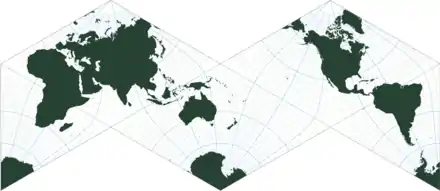
The Dixon elliptic functions are conformal maps from an equilateral triangle to a disk, and are therefore helpful for constructing polyhedral conformal map projections involving equilateral triangles, for example projecting the sphere onto a triangle, hexagon, tetrahedron, octahedron, or icosahedron.[15]

External links

Desmos plots:
- Real-valued Dixon elliptic functions https://www.desmos.com/calculator/5s4gdcnxh2.
- Parametrizing the cubic Fermat curve, https://www.desmos.com/calculator/elqqf4nwas
On-Line Encyclopedia of Integer Sequences pages:
- “Coefficient of x^(3n+1)/(3n+1)! in the Maclaurin expansion of the Dixon elliptic function sm(x,0).” https://oeis.org/A104133
- “Coefficient of x^(3n)/(3n)! in the Maclaurin expansion of the Dixon elliptic function cm(x,0).” https://oeis.org/A104134
- “Pi(3): fundamental real period of the Dixonian elliptic functions sm(z) and cm(z).” https://oeis.org/A197374
Mathematics Stack Exchange discussions:
- “On $x^{3}+y^{3}=z^{3}$ , the Dixonian elliptic functions, and the Borwein cubic theta functions”, https://math.stackexchange.com/questions/2090523/
- “doubly periodic functions as tessellations (other than parallelograms)”, https://math.stackexchange.com/questions/35671/

Notes

Dark areas represent zeros, and bright areas represent poles. As the argument of $\operatorname {sm} z$ changes from $-\pi$ (excluding $-\pi$ ) to $\pi$ , the colors go through cyan, blue ( $\operatorname {Arg} \approx -\pi /2$ ), magneta, red ( $\operatorname {Arg} \approx 0$ ), orange, yellow ( $\operatorname {Arg} \approx \pi /2$ ), green, and back to cyan ( $\operatorname {Arg} \approx \pi$ ).
Dixon (1890), Dillner (1873). Dillner uses the symbols $W=\operatorname {sm} ,\ W_{1}=\operatorname {cm} .$
Dixon (1890), Van Fossen Conrad & Flajolet (2005), Robinson (2019).
The mapping for a general regular polygon is described in Schwarz (1869).
van Fossen Conrad & Flajolet (2005) p. 6.
Dillner (1873) calls the period $3w$ . Dixon (1890) calls it $3\lambda$ ; Adams (1925) and Robinson (2019) each call it $3K$ . Van Fossen Conrad & Flajolet (2005) call it $\pi _{3}$ . Also see OEIS A197374.
Dixon (1890), Van Fossen Conrad & Flajolet (2005)
Dixon (1890), Adams (1925)
Adams (1925)
van Fossen Conrad & Flajolet (2005). Also see OEIS A104133, A104134.
Reinhardt & Walker (2010)
Chapling (2018), Robinson (2019). Adams (1925) instead expresses the Dixon elliptic functions in terms of the Weierstrass elliptic function $\wp (z;0,-1).$
van Fossen Conrad & Flajolet (2005), p.38
Lundberg (1879), Grammel (1948), Shelupsky (1959), Burgoyne (1964), Gambini, Nicoletti, & Ritelli (2021).
Adams (1925), Cox (1935), Magis (1938), Lee (1973), Lee (1976), McIlroy (2011), Chapling (2016).

References

O. S. Adams (1925). Elliptic functions applied to conformal world maps (No. 297). US Government Printing Office. ftp://ftp.library.noaa.gov/docs.lib/htdocs/rescue/cgs_specpubs/QB275U35no1121925.pdf
R. Bacher & P. Flajolet (2010) “Pseudo-factorials, elliptic functions, and continued fractions” The Ramanujan journal 21(1), 71–97. https://arxiv.org/pdf/0901.1379.pdf
A. Cayley (1882) “Reduction of ${\textstyle \int dx/(1-x^{3}){}^{2/3}}$ to elliptic integrals”. Messenger of Mathematics 11, 142–143. https://gdz.sub.uni-goettingen.de/id/PPN599484047_0011?tify={%22pages%22:%5b146%5d}
F. D. Burgoyne (1964) “Generalized trigonometric functions”. Mathematics of Computation 18(86), 314–316. https://www.jstor.org/stable/2003310
A. Cayley (1883) “On the elliptic function solution of the equation $x 3 + y 3 - 1 = 0$ ”, Proceedings of the Cambridge Philosophical Society 4, 106–109. https://archive.org/details/proceedingsofcam4188083camb/page/106/
R. Chapling (2016) “Invariant Meromorphic Functions on the Wallpaper Groups”. https://arxiv.org/pdf/1608.05677
J. F. Cox (1935) “Répresentation de la surface entière de la terre dans une triangle équilatéral”, Bulletin de la Classe des Sciences, Académie Royale de Belgique 5e, 21, 66–71.
G. Dillner (1873) “Traité de calcul géométrique supérieur”, Chapter 16, Nova acta Regiae Societatis Scientiarum Upsaliensis, Ser. III 8, 94–102. https://archive.org/details/novaactaregiaeso38kung/page/94/
Dixon, A. C. (1890). "On the doubly periodic functions arising out of the curve $x 3 + y 3 - 3 αxy = 1$ ". Quarterly Journal of Pure and Applied Mathematics. XXIV: 167–233.
A. Dixon (1894) The elementary properties of the elliptic functions. MacMillian. https://archive.org/details/elempropellipt00dixorich/
Van Fossen Conrad, Eric; Flajolet, Philippe (2005). "The Fermat cubic, elliptic functions, continued fractions, and a combinatorial excursion". Séminaire Lotharingien de Combinatoire. 54: Art. B54g, 44. arXiv:math/0507268. Bibcode:2005math......7268V. MR 2223029.
A. Gambini, G. Nicoletti, & D. Ritelli (2021) “Keplerian trigonometry”. Monatshefte für Mathematik 195(1), 55–72. https://doi.org/10.1007/s00605-021-01512-0
R. Grammel (1948) “Eine Verallgemeinerung der Kreis-und Hyperbelfunktionen”. Archiv der Mathematik 1(1), 47–51. https://doi.org/10.1007/BF02038206
J. C. Langer & D. A. Singer (2014) “The Trefoil”. Milan Journal of Mathematics 82(1), 161-182. https://case.edu/artsci/math/langer/jlpreprints/Trefoil.pdf
M. Laurent (1949) “Tables de la fonction elliptique de Dixon pour l’intervalle 0-0, 1030”. Bulletin de l’Académie Royale des Sciences de Belgique Classe des Sciences, 35, 439–450.
L. P. Lee (1973) “The Conformal Tetrahedric Projection with some Practical Applications”. The Cartographic Journal, 10(1), 22-28. https://doi.org/10.1179/caj.1973.10.1.22
L. P. Lee (1976) Conformal Projections Based on Elliptic Functions. University of Toronto Press. Cartographica Monograph No. 16.
E. Lundberg (1879) “Om hypergoniometriska funktioner af komplexa variabla”. Manuscript, 1879. Translation by Jaak Peetre “On hypergoniometric functions of complex variables”. https://web.archive.org/web/20161024183030id_/http://www.maths.lth.se/matematiklu/personal/jaak/hypergf.ps
J. Magis (1938) “Calcul du canevas de la représentation conforme de la sphère entière dans un triangle équilatéral”. Bulletin Géodésique 59(1), 247–256. http://doi.org/10.1007/BF03029866
M. D. McIlroy (2011) “Wallpaper maps”. Dependable and Historic Computing. Springer. 358–375. https://link.springer.com/chapter/10.1007/978-3-642-24541-1_27
W. P. Reinhardt & P. L. Walker (2010) “Weierstrass Elliptic and Modular Functions”, NIST Digital Library of Mathematical Functions, §23.5(v). https://dlmf.nist.gov/23.5#v
P. L. Robinson (2019) “The Dixonian elliptic functions”. https://arxiv.org/abs/1901.04296
H. A. Schwarz (1869) “Ueber einige Abbildungsaufgaben”. Crelles Journal 1869(70), 105–120. http://doi.org/10.1515/crll.1869.70.105
B. R. Seth & F. P. White (1934) “Torsion of beams whose cross-section is a regular polygon of n sides”. Mathematical Proceedings of the Cambridge Philosophical Society, 30(2), 139. http://doi.org/10.1017/s0305004100016558
D. Shelupsky (1959) “A generalization of the trigonometric functions”. The American Mathematical Monthly 66(10), 879–884. https://www.jstor.org/stable/2309789

This article is issued from Wikipedia. The text is licensed under Creative Commons - Attribution - Sharealike. Additional terms may apply for the media files.

[1] Dark areas represent zeros, and bright areas represent poles. As the argument of $\operatorname {sm} z$ changes from $-\pi$ (excluding $-\pi$ ) to $\pi$ , the colors go through cyan, blue ( $\operatorname {Arg} \approx -\pi /2$ ), magneta, red ( $\operatorname {Arg} \approx 0$ ), orange, yellow ( $\operatorname {Arg} \approx \pi /2$ ), green, and back to cyan ( $\operatorname {Arg} \approx \pi$ ).

[2] Dixon (1890), Dillner (1873). Dillner uses the symbols $W=\operatorname {sm} ,\ W_{1}=\operatorname {cm} .$

[3] Dixon (1890), Van Fossen Conrad & Flajolet (2005), Robinson (2019).

[4] The mapping for a general regular polygon is described in Schwarz (1869).

[5] van Fossen Conrad & Flajolet (2005) p. 6.

[6] Dillner (1873) calls the period $3w$ . Dixon (1890) calls it $3\lambda$ ; Adams (1925) and Robinson (2019) each call it $3K$ . Van Fossen Conrad & Flajolet (2005) call it $\pi _{3}$ . Also see OEIS A197374.

[7] Dixon (1890), Van Fossen Conrad & Flajolet (2005)

[8] Dixon (1890), Adams (1925)

[9] Adams (1925)

[10] van Fossen Conrad & Flajolet (2005). Also see OEIS A104133, A104134.

[11] Reinhardt & Walker (2010)

[12] Chapling (2018), Robinson (2019). Adams (1925) instead expresses the Dixon elliptic functions in terms of the Weierstrass elliptic function $\wp (z;0,-1).$

[13] van Fossen Conrad & Flajolet (2005), p.38

[14] Lundberg (1879), Grammel (1948), Shelupsky (1959), Burgoyne (1964), Gambini, Nicoletti, & Ritelli (2021).

[15] Adams (1925), Cox (1935), Magis (1938), Lee (1973), Lee (1976), McIlroy (2011), Chapling (2016).